Archive
Python: Machine Learning – Part 1
Learning :Python and Machine Learning
Subject: Requirements, Sample and Implementation
Machine Learning: I will not go through definitions and uses of ML, I think there is a lot of other posts that may be more informative than whatever i will write. In this post I will write about my experience and learning carve to learn and implement ML model and test my own data.
The Story: Two, three days ago I start to read and watch videos about Machine Learning, I fond the “scklearn” site, from there I create the first ML to test an Iris data-set and then I wrote a function to generate data (my own random data) and test it with sklearn ML model.
Let’s start ..
Requirements:
1. Library to Import: To work with sklearn models and other functions that we will use, we need to import coming libraries:
import os # I will use it to clear the terminal.
import random # I will use it to generate my data-set.
import numpy as np
import bunch # To create data-set as object
from sklearn import datasets
from sklearn import svm
from sklearn import tree
from sklearn.model_selection import train_test_split as tts
2. Data-set: In my learning steps I use one of sklearn data-set named ” Iris” it store information about a flower called ‘Iris’. To use sklear ML Model on other data-sets, I create several functions to generate random data that can be passed into the ML, I will cover this part later in another post.
First we will see what is the Iris dataset, this part of information is copied from sklearn site.
::Iris dataset description ::
dataset type: Classification
contain: 3 classes, 50 Samples per class (Total of 150 sample)
4 Dimensionality
Features: real, positive
The data is Dictionary-like object, the interesting attributes are:
‘data’: the data to learn.
‘target’: the classification labels.
‘target_names’: the meaning of the labels.
‘feature_names’: the meaning of the features.
‘DESCR’: the full description of the dataset.
‘filename’: the physical location of iris csv.
Note: This part helps me to write me data-set generating function, that’s why we import the Bunch library to add lists to a data-set so it will appear as an object data-set, so the same code we use for Iris data-set will work fine with our data-set. In another post I will cover I will load the data from csv file and discover how to create a such file..
Start Writing the code parts: After I wrote the code and toned it, I create several functions to be called with other data-set and not hard-code any names in iris data-set. This way we can load other data-set in easy way.
The Code
 # import libraries

import numpy as np
from sklearn import datasets
#from sklearn import svm
from sklearn import tree
from sklearn.model_selection import train_test_split as tts
import random, bunch
Next step we will load the iris dataset into a variable called “the_data”
 # loading the iris dataset.

the_data = datasets.load_iris()
From the above section “Iris dataset description” we fond that the data is stored in data, and the classification labels stored in target, so now we will store the data and the target in another two variables.
 # load the data into all_data, and target in all_labels.
all_data= the_data.data
all_labels = the_data.target
We will create an object called ‘clf’ and will use the Decision Tree Classifier from sklearn.
 #  create Decision Tree Classifier

clf = tree.DecisionTreeClassifier()
In Machine Learning programs, we need some data for training and another set of data for testing before we pass the original data or before we deploy our code for real data. The sklearn providing a way or say function to split a given data into two parts test and train. To do this part and to split the dataset into training and test I create a function that we will call and pass data and label set to it and it will return the following : train_data, test_data, train_labels, test_labels.
 #  Function to split a data-set into training and testing data.

def get_test_train_data(data,labels):

  train_data, test_data, train_labels, test_labels = tts(data,labels,test_size = 0.1)
  return train_feats, test_feats, train_labels, test_labels
After splitting the data we will have four list or say data-sets, we will pass the train_data and the train_labels to the train_me() function, I create this function so we can pass the train_data, train_labels and it will call the (clf.fit) from sklearn. By finishing this part we have trained our ML Model and is ready to test a sample data. But first let’s see the train_me() function.
 #  Function train_me() will pass the train_data to sklearn Model.

def train_me(train_data1,train_labels1):
  clf.fit(train_data1,train_labels1)
  print('\n The Model been trained. ')
As we just say, now we have a trained Model and ready for testing. To test the data set we will use the clf.predict function in sklearn, this should return a prediction labels list as the ML Model think that is right. To check if the predictions of the Model is correct or not also to have the percentage of correct answers we will count and compare the prediction labels with the actual labels in the test_data that we have. Here is the code for get_prediction()
 #  get_prediction() to predict the data labels.

def get_prediction(new_data_set,test_labels2,accu):

  print('\n This is the prediction labels of the data.\n')

  # calling prediction function clf.predict
  prediction = clf.predict(new_data_set)
  print('\n prediction labels are : ',prediction,len(prediction))

  # print the Accuracy
  if accu == 't' :
    cot = 0
    for i in range (len(prediction)) :
      print(prediction[i] , new_data_set[i],test_labels2[i])
      if [prediction[i]] == test_labels2[i]:
        cot = cot + 1
    print('\ncount :',cot)
    print('\n The Accuracy:',(cot/len(prediction))*100,'%')
The accuracy value determine if we can use the model in a real life or tray to use other model. In the real data scenario, we need to pass ‘False’ flag for accu, because we can’t cross check the predicted result with any data, we can try to check manually for some result.
End of part 1: by now, we have all functions that we can use with our data-set, in coming images of the code and run-time screen we can see that we have a very high accuracy level so we can use our own data-set, and this will be in the coming post.

|
Result screen shot after running the Iris dataset showing high accuracy level.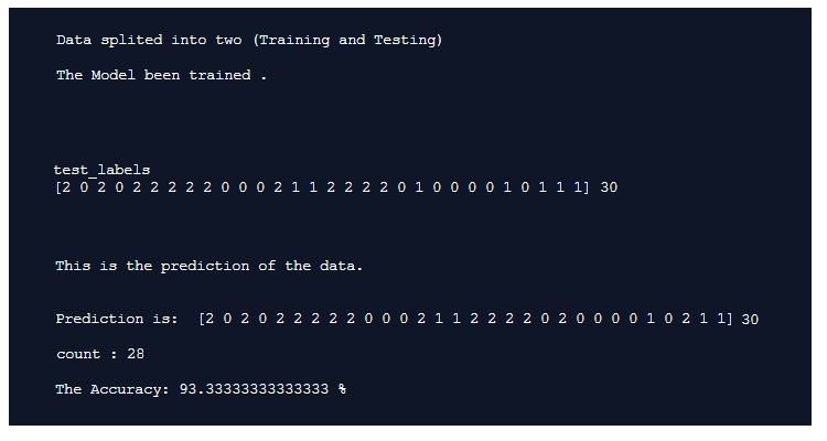
|
To Download my Python code (.py) files Click-Here
 Follow me on Twitter..
Python ploting
Learning : Plotting Data using python and numpy
Subject: Plotting Data
The best way to show the data is to make them as a graph or charts, there are several charts type and names each will present your data in a different way and used for different purpose. Plotting the data using python is a good way to show out your data and in coming posts we will cover very basic aspects in plotting data. So if we just want to show a sample for what we are talking about, we will say: we have a sample of hospital data for born childs (male m, female f, in years 200 to 2003).
:: Click to enlarge :: 
|
There are some libraries we can use in python to help us plotting the data, here are some of them. Matplotlib, Plotly and Seaborn are just samples of what we may use, in this post we will use the Matplotlib. To use Matplotlib we need to install it, so if it is not installed in your python you need to do so.
pip install Matplotlib
Then we need to import it in our code using :
import matplotlib.pyplot as plt
To show the data we need to have some variables that will be used in our first example, So the case is that we have some data from a hospital, the data are numbers of born childs (male m, female f) in years 2000 to 2003. We will store/save the data in list, we will have data_yesrs =[2000,2001,2002,2003], then we will have male born data in data_m=[2,2.5,3,5] and female born data data_f = [3,3.8,4,4.5], the chart will have two axis vertical is Y y_data_title =’In Hundreds’ and horizontal is X x_data_title =’ Years’, now to project all this information on a chart we use this code ..
import matplotlib.pyplot as plt
data_yesrs = [2000,2001,2002,2003] # years on X axis
data_m = [2,2.5,3,5]   # y data males born
data_f = [3,3.8,4,4.5]  # y data female born
y_data_title ='In Thousands'
x_data_title =' Years'

plt.title('New Born babies')

plt.plot(data_yesrs,data_m,'r-', data_yesrs,data_f,'b--')
plt.ylabel(y_data_title)
plt.xlabel(x_data_title)
plt.show()
Another way to plot the data were we can use a one line for each data set as:
plt.plot(data_x,data_m,’r-‘)
plt.plot(data_x,data_f,’b–‘)
We can see that male data is red line, and female data is blue dashes, we can use some line style to present the data as mentioned bellow:
‘-‘ or ‘solid’ is solid line
‘–‘ or ‘dashed’ is dashed line
‘-.’ or ‘dashdot’ is dash-dotted line
‘:’ or ‘dotted’ is dotted line
‘None’ or ‘ ‘ or ” is draw nothing
And also we can use colors such as :
r: red, g: green,
b: blue, y: yellow .
If we want to add the map or chart key, we need first to import matplotlib.patches as mpatches then to add this line of code:
plt.legend([‘Male’,’Female’])
and the keys [‘Male’,’Female’] MUST be in the same sequence as the main plot code line :
plt.plot(data_yesrs,data_m,’r-‘, data_yesrs,data_f,’b–‘)

|
To Download my Python code (.py) files Click-Here
Python: Circle Packing
Circle Packing Project
Subject: Draw, circles, Turtle
Definition: In geometry, circle packing is the study of the arrangement of circles on a given surface such that no overlapping occurs and so that all circles touch one another. Wikipedia
So, we have a canvas size (w,h) and we want to write a code to draw X number of circles in this area without any overlapping or intersecting between circles. We will write some functions to do this task, thous functions are:
1. c_draw (x1,y1,di): This function will take three arguments x1,y1 for circle position and di as circle diameter.
2. draw_fram(): This function will draw the frame on the screen, we set the frame_w and frame_h as variables in the setup area in the code.
3. c_generator (max_di): c_generator is the circles generating function, and takes one argument max_di presenting the maximum circles diameter. To generate a circle we will generate three random numbers for x position, y position and for circle diameter (max_di is the upper limit),also with each generating a while loop will make sure that the circle is inside the frame, if not regenerate another one.
4. can_we_draw_it (q1,di1): This is very important, to make sure that the circle is not overlapping with any other we need to use a function call (hypot) from math library hypot return the distance between two points, then if the distance between two circles is less than the total of there diameters then the two circles are not overlaps.

|
So, lets start coding …
First: the import and setup variables:
from turtle import *
import random
import math

# Create a turtle named t:
t =Turtle()
t.speed(0)
t.hideturtle()
t.setheading(0)
t.pensize(0.5)
t.penup()

# frame size
frame_w = 500
frame_h = 600

di_list = [] # To hold the circles x,y and diameters
 |
Now, Drawing the frame function:
def draw_fram () :t.penup()
t.setheading(0)
t.goto(-frame_w/2,frame_h/2)
t.pendown()
t.forward(frame_w)
t.right(90)
t.forward(frame_h)
t.right(90)
t.forward(frame_w)
t.right(90)
t.forward(frame_h)
t.penup()
t.goto(0,0)
Now, Draw circle function:
def c_draw (x1,y1,di):t.goto(x1,y1)
t.setheading(-90)
t.pendown()
t.circle(di)
t.penup()
This is Circles generator, we randomly select x,y and diameter then checks if it is in or out the canvas.
def c_generator (max_di):falls_out_frame = True
while falls_out_frame :
x1 = random.randint(-(frame_w/2),(frame_w/2))
y1 = random.randint(-(frame_h/2),(frame_h/2))
di = random.randint(3,max_di)
# if true circle is in canvas
if (x1-di > ((frame_w/2)*-1)) and (x1-di < ((frame_w/2)-(di*2))) :
if (y1 ((frame_h/2)-(di))*-1) :
falls_out_frame = False
di_list.append([x1-di,y1,di])

|
With each new circle we need to check the distances and the diameter between new circle and all circles we have in the list, if there is an overlap then we delete the new circle data (using di_list.pop()) and generate a new circle. So to get the distances and sum of diameters we use this code ..
 # get circles distance

    cs_dis = math.hypot(((last_cx + last_cdi) - (c_n_list_x + c_n_list_di)) , (last_cy - c_n_list_y))
    di_total = last_cdi + c_n_list_di
To speed up the generation of right size of circles I use a method of counting the trying times of wrong sizes, that’s mean if the circles is not fit, and we pop it’s details from the circles list we count pops, if we reach certain number then we reduce the upper limits of random diameter of the new circles we generate. Say we start with max_di = 200, then if we pop for a number that divide by 30 (pop%30) then we reduce the max_di with (-1) and if we reach max_di less then 10 then max_di = 60. and we keep doing this until we draw 700 circles.
# if di_list pops x time then we reduce the randomization upper limits
  if (total_pop % 30) == 0:
    max_di = max_di - 1
    if max_di < 10 :
      max_di = 60
Here are some output circles packing ..
 |
 |
With current output we reach the goal we are looking for, although there is some empty spaces, but if we increase the number of circles then there will be more time finding those area with random (x,y,di) generator, I am thinking in another version of this code that’s will cover:
1. Coloring the circles based on the diameter size.
2. A method to fill the spaces.
To Download my Python code (.py) files Click-Here
Python: Numpay – P3
Learning : Python Numpy – P3
Subject: numpy array and some basic commands
The numpy lessons and basic commands will take us to plotting the data and presenting the numbers using the numpy and plot packages, but first we need to do more practices on arrays and functions in the numpy.
To get a row or a column from the array we use:
# Generate a 5x5 random array:
ar = np.random.randint(10,60, size=(5,5))
print('\n A random generated array 5x5 is: \n',ar)

# get the rows from 1 to 3 (rows 1 and 2):
print('\n  The rows from 1 to 3 is: \n',ar[1:3])

# get row 1 and row 3:
print('\n  The row 1 and row 2 is: \n',ar[1],ar[3])

# get the column 1 and column 3:
print('\n  The column 1 and column 3: \n',ar[:,[1,3]])

[Output]:
A random generated array 5x5 is:
 [[59 43 46 44 39]
 [16 15 14 19 22]
 [59 16 33 59 19]
 [21 15 51 41 28]
 [48 46 58 33 19]]

The rows from 1 to 3 is:
[[16 15 14 19 22]
 [59 16 33 59 19]]

The row 1 and row 2 is:
[16 15 14 19 22]
[21 15 51 41 28]

The column 1 and column 3:
 [[43 44]
 [15 19]
 [16 59]
 [15 41]
 [46 33]]
To change a value in the array we give the position and new value as:
# Generate a 5x5 random array:
ar = np.random.randint(10,60, size=(5,5))
print('\n A random generated array 5x5 is: \n',ar)
print('\n Value in position (1,1):',ar[1][1])
# Re-set the value in position (1,1) to 55
ar[1][1] = 55
print('\n The array ar\n',ar)

code
[Output]:

A random generated array 5x5 is:
 [[39 53 34 59 30]
 [33 10 42 20 36]
 [10 37 20 35 28]
 [26 18 14 41 24]
 [48 22 19 18 44]]

 Value in position (1,1): 10

 The array ar
 [[39 53 34 59 30]
 [33 55 42 20 36]
 [10 37 20 35 28]
 [26 18 14 41 24]
 [48 22 19 18 44]]
If we have a one dimension array with values, and we want to create another array with values after applying a certain conditions, such as all values grater than 7.
# Create 1D array of range 10
ar = np.arange(10)
print(ar)

# ar_g7 is a sub array from ar of values grater then 7
ar_g7= np.where(ar >7)
print('ar_g7:'ar_g7)


[Output]:
[0 1 2 3 4 5 6 7 8 9]
ar_g7:(array([8, 9]),)
If we want to pass a 3×3 array and then we want the values to be changed to (1) if it is grater than 7 and to be (0) if it is less than 7.
# Generate a 3x3 array of random numbers.
ar2 = np.random.randint(1,10, size =(3,3))
print(ar2)

# Change any value grater than 7 to 1 and if less than 7 to 0.
ar_g7= np.where(ar2 >7, 1 ,0)
print('ar_g7:',ar_g7)

[Output]:
[[6 4 2]
 [8 5 1]
 [5 2 8]]

ar_g7:
[[0 0 0]
 [1 0 0]
 [0 0 1]]
Also we can say if, the value in the array is equal to 6 or 8 then change it to -1.
# Generate array of 3x3
ar2 = np.random.randint(1,10, size =(3,3))
print(ar2)


# If the = 6 or 8 change it to (-1)
ar_get_6_8_value= np.where((ar2 == 6) |( ar2==8), -1 ,ar2)
print('ar_get_6_8_value:',ar_get_6_8_value)

[Output]:
[[3 4 8]
 [1 9 3]
 [5 6 6]]

ar_get_6_8_value:
[[ 3  4 -1]
[ 1  9  3]
[ 5 -1 -1]]
We can get the index location of the certain conditions values, and then we can print it out.
# # Generate array of 3x3

ar_less_6= np.where((ar2 < 6) )
print('ar_less_6 locations:',ar_less_6)

# print out the values on those locations.
print('ar_less_6 values: ',ar2[ar_less_6])
[Output]:
[[6 1 9]
 [1 8 6]
 [6 9 2]]

ar_less_6 locations: (array([0, 1, 2]), array([1, 0, 2]))
ar_less_6 values :[1 1 2]
:: numpy Sessions ::
| Sessions 1 | Sessions 2 | Sessions 3 | Sessions 4 |
To Download my Python code (.py) files Click-Here
Python: Numpay – P2
Learning : Python Numpy – P2
Subject: Two Dimensional array and some basic commands
In real mathematics word we mostly using arrays with more than one dimensions, for example with two dimension array we can store a data as
So let’s start, if we want to create an array with 24 number in it starting from 0 to 23 we use the command np.range. as bellow :
 # We are using np.range to create an array of numbers between (0-23)

m_array = np.arange(24)
print(m_array)
[Output]:
[ 0  1  2  3  4  5  6  7  8  9 10 11 12 13 14 15 16 17 18 19 20 21 22 23]
And if we want the array to be in a range with certain incriminating amount we may use this command:
 # Create array between 2-3 with 0.1 interval

m_array = np.arange(2, 3, 0.1)
print(m_array)
[Output]:
[ 2. , 2.1, 2.2, 2.3, 2.4, 2.5, 2.6, 2.7, 2.8, 2.9]
Now if we want to create an array say 3×3 fill with random numbers from (0-10) we use random function in numpy as bellow:
 # create 3x3 Array with random numbers 0-10
m_array = np.random.randint(10, size=(3,3))
print(m_array)
[Output]:
[[6 0 7]
 [1 9 8]
 [5 8 9]]

|
And if we want the random number ranges to be between two numbers we use this command:
# Array 3x3 random values between (10-60)
m_array = np.random.randint(10,60, size=(3,3))
[Output]:
[[11 23 50]
 [36 44 18]
 [56 24 30]]
If we want to reshape the array; say from 4×5 (20 element in the array) we can reshape it but with any 20-element size. Here is the code:
# To crate a randome numbers in an array of 4x5 and numbers range 10-60.
m_array = np.random.randint(10,60, size=(4,5))
print(m_array)

# We will reshape the 4x5 to 2x10
new_shape = m_array.reshape(2,10)
print ('\n   Tne new 2x10 array:\n',new_shape)
[Output]:
[[37 11 56 18 42]
 [17 12 22 16 42]
 [47 29 17 47 35]
 [49 55 43 13 11]]

Tne new 2x10 array:
[[37 11 56 18 42 17 12 22 16 42]
 [47 29 17 47 35 49 55 43 13 11]]
Also we can convert a list to an array,
# Convert a list l=([2,4,6,8]) to a 1D array
# l is a list with [2,4,6,8] values.
l=([2,4,6,8])
print('  l= ',l)
# Convert it to a 1D array.
ar = np.array(l)
print('\n  Type of l:',type(l),', Type of ar:',type(ar))
print('  ar = ',ar)

[Output]:
l=  [2, 4, 6, 8]
Type of: class'list'  , Type of ar: class 'numpy.ndarray'
ar =  [2 4 6 8]
If we want to add a value to all elements in the array, we just write:
# Adding 9 to each element in the array


print('ar:',ar)
ar = ar + 9
print('ar after adding 9:',ar)

[Output]:
ar:  [2 4 6 8]
ar after adding 9: [11 13 15 17]
:: numpy Commands::
| Command | Comments and Outputs |
| my_array = np.array([1,2,3,4,5]) | Create an array with 1 to 5 integer |
| len(my_array) | Get the array length |
| np.sum(my_array) | get the sum of the elements in the array my_array = np.array([1,2,3,4,5]) print(np.sum(my_array)) [Output]: 15 |
| np.max(my_array) | # Get the maximum number in the array my_array = np.array([1, 2, 3,4,5]) max_num = np.max(my_array) [Output]: 5 |
| np.min(my_array) | # Get the minimum number in the array my_array = np.array([1, 2, 3,4,5]) min_num = np.min(my_array) [Output]: 1 |
|
my_array = np.ones(5) Output: [ 1., 1., 1., 1., 1.] |
create array of 1s (of length 5) np.ones(5) Output: [ 1., 1., 1., 1., 1.] |
| m_array = np.arange(24) print(m_array) |
# To create an array with 23 number. [ 0 1 2 3 4 5 6 7 8 9 10 11 12 13 14 15 16 17 18 19 20 21 22 23] |
| m_array = np.arange(2, 3, 0.1) print(m_array) |
# Create an array from 2 to 3 with 0.1 interval value increments. [ 2. , 2.1, 2.2, 2.3, 2.4, 2.5, 2.6, 2.7, 2.8, 2.9] |
| m_array = np.random.randint(10, size=(3,3)) print(m_array) |
# Create a 3×3 array with random numbers between (0,10) [[6 0 7] [1 9 8] [5 8 9]] |
| m_array = np.random.randint(10,60, size=(3,3)) | # Create a 3×3 array with random numbers between (10,60) [[11 23 50] [36 44 18] [56 24 30]] |
| # Create a 4×5 array with random numbers. m_array = np.random.randint(10,60, size=(4,5)) # Reshape m_array from 4×5 to 2×10 |
# m_array 4×5 [[37 11 56 18 42] [17 12 22 16 42] [47 29 17 47 35] [49 55 43 13 11]] # Tne new 2×10 array: |
| # convert a list to array: l=[2,4,6,8] ar = np.array(l) # check data type for l and ar: print(‘\n Type of l:’,type(l),’, Type of ar:’,type(ar)) |
[Output]: l = [2, 4, 6, 8] ar = [2, 4, 6, 8] Type of l: class ‘list,’, Type of ar: class ‘numpy.ndarray’ |
| # Adding 9 to each element in the array ar = ar + 9 |
[11 13 15 17] |
:: numpy Sessions ::
| Sessions 1 | Sessions 2 | Sessions 3 | Sessions 4 |
:: Some Code output ::
Create array with 24 numbers (0-23).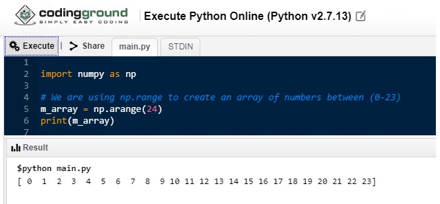
|
Reshape array to 4×6. |
| Create random array of numbers (0-10), size 3×3. |
Reshape 4×5 array to 2×10. |
Convert list to array.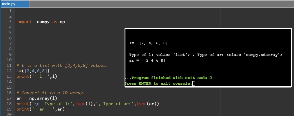 |
To Download my Python code (.py) files Click-Here
Python: Numpay – P1
Learning : Python Numpy – P1
Subject: Numpay and some basic commands
In coming several posts I will talk about the numpay library and how to use some of its functions. So first what is numpy? Definition: NumPy is a library for the Python programming language, adding support for large, multi-dimensional arrays and matrices, along with a large collection of high-level mathematical functions to operate on these arrays. Also known as powerful package for scientific computing and data manipulation in python. As any library or package in python we need to install it on our device (we will not go through this process)
Basic commands in numpy: First of all we need to import it in our code. so we will use
import numpy as np
To create a 1 dimensional array we can use verey easy way as:
  # create an array using numpy array function.
my_array = np.array([1, 2, 3,4,5])
Later we will create a random array of numbers in a range.
Now, to get the length of the array we can use len command as
len(my_array)
Output: 5
To get the sum of all elements in the array we use..
np.sum(my_array)
And to get the maximum and minimum numbers in the array we use ..
 # Get the maximum and minimum numbers in the array
my_array = np.array([1, 2, 3,4,5])
np.max(my_array)
[Output]: 5

np.min(my_array)
[Output]: 1
Some time we may need to create an array with certain Number of elements only one’s, to do this we can use this commands:
#create array of 1s (of length 5)
np.ones(5)
Output: [ 1.,  1.,  1.,  1.,  1.]
The default data type will be float, if we want to change it we need to pass the the ‘dtype’ to the command like this :
#create array of 1s (of length 5) as integer:
np.ones(5, dtype = np.int)
Output: [ 1,  1,  1,  1,  1]
Code output:

|
So far we work on a one dimensional array, in the next post we will cover some commands that will help us in the arrays with multiple dimensions.
:: numpy Commands::
| Command | comment |
| my_array = np.array([1,2,3,4,5]) | Create an array with 1 to 5 integer |
| len(my_array) | Get the array length |
| np.sum(my_array) | get the sum of the elements in the array my_array = np.array([1,2,3,4,5]) print(np.sum(my_array)) [Output]: 15 |
| np.max(my_array) | # Get the maximum number in the array my_array = np.array([1, 2, 3,4,5]) max_num = np.max(my_array) [Output]: 5 |
| np.min(my_array) | # Get the minimum number in the array my_array = np.array([1, 2, 3,4,5]) min_num = np.min(my_array) [Output]: 1 |
|
my_array = np.ones(5) Output: [ 1., 1., 1., 1., 1.] |
create array of 1s (of length 5) np.ones(5) Output: [ 1., 1., 1., 1., 1.] |
:: numpy Sessions ::
| Sessions 1 | Sessions 2 | Sessions 3 | Sessions 4 |
To Download my Python code (.py) files Click-Here
Python and Lindenmayer System – P3
Learning : Lindenmayer System P3
Subject: Drawing Fractal Tree using Python L-System
In the first two parts of the L-System posts (Read Here: P1, P2) we talk and draw some geometric shapes and patterns. Here in this part 3 we will cover only the Fractal Tree and looking for other functions that we may write to add leaves and flowers on the tree.
Assuming that we have the Pattern generating function and l-system drawing function from part one, I will write the rules and attributes to draw the tree and see what we may get.
So, first tree will have:
# L-System Rule to draw ‘Fractal Tree’
# Rule: F: F[+F]F[-F]F
# Angle: 25
# Start With: F
# Iteration : 4
and the output will be this:

|
If we need to add some flowers on the tree, then we need to do two things, first one is to write a function to draw a flower, then we need to add a variable to our rule that will generate a flower position in the pattern. First let’s write a flower function. We will assume that we may want just to draw a small circles on the tree, or we may want to draw a full open flower, a simple flower will consist of 4 Petals and a Stamen, so our flower drawing function will draw 4 circles to present the Petals and one middle circle as the Stamen. We will give the function a variable to determine if we want to draw a full flower or just a circle, also the size and color of the flowers.
Here is the code ..
font = 516E92
commint = #8C8C8C
Header here
# Functin to draw Flower
def d_flower () :
if random.randint (1,1) == 1 :
# if full_flower = ‘y’ the function will draw a full flower,
# if full_flower = ‘n’ the function will draw only a circle
full_flower = ‘y’
t.penup()
x1 = t.xcor()
y1 = t.ycor()
f_size = 2
offset = 3
deg = 90
if full_flower == ‘y’ :
t.color(‘#FAB0F4’)
t.fillcolor(‘#FAB0F4’)
t.goto(x1,y1)
t.setheading(15)
for x in range (0,4) : # To draw a 4-Petals
t.pendown()
t.begin_fill()
t.circle(f_size)
t.end_fill()
t.penup()
t.right(deg)
t.forward(offset)
t.setheading(15)
t.goto(x1,y1 – offset * 2 + 2)
t.pendown() # To draw a white Stamen
t.color(‘#FFFFF’)
t.fillcolor(‘#FFFFFF’)
t.begin_fill()
t.circle(f_size)
t.end_fill()
t.penup()
else: # To draw a circle as close flower
t.pendown()
t.color(‘#FB392C’)
t.end_fill()
t.circle(f_size)
t.end_fill()
t.penup()
t.color(‘black’)
Then we need to add some code to our rule and we will use variable ‘o’ to draw the flowers, also I will add a random number selecting to generate the flowers density. Here is the code for it ..
In the code the random function will pick a number between (1-5) if it is a 3 then the flower will be drawn. More density make it (1-2), less density (1-20)
|
And here is the output if we run the l-System using this rule: Rule: F: F[+F]F[-F]Fo

|
Using the concepts, here is some samples with another Fractal Tree and flowers.
Another Fractal Tree without any Flowers.
|
Fractal Tree with closed Pink Flowers.
|
Fractal Tree with closed Red Flowers.
|
Fractal Tree with open pink Flowers.
|
To Download my Python code (.py) files Click-Here
Python and Lindenmayer System – P2
Learning : Lindenmayer System P2
Subject: Drawing with python using L-System
In the first part of Lindenmayer System L-System post (Click to Read) we had wrote two functions: one to generate the pattern based on the variables and roles, and one to draw lines and rotate based on the pattern we have.
In this part I will post images of what Art we can generate from L-System
the codes will be the L-system that generate the patterns, so the code will include: the Rules, Angle (Right, Left) Iteration and Starting Variable.
 |
L-System: Koch Curve  |
L-System: Minkowski Sausage |
L-System: … but here the Iteration is: 3 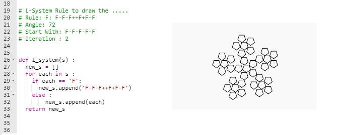 |
L-System: Again … but here the Iteration is: 3  |
L-System: Square Sierpinski  |
L-System: Sierpinski Arrowhead.  |
L-system: Dragon Curve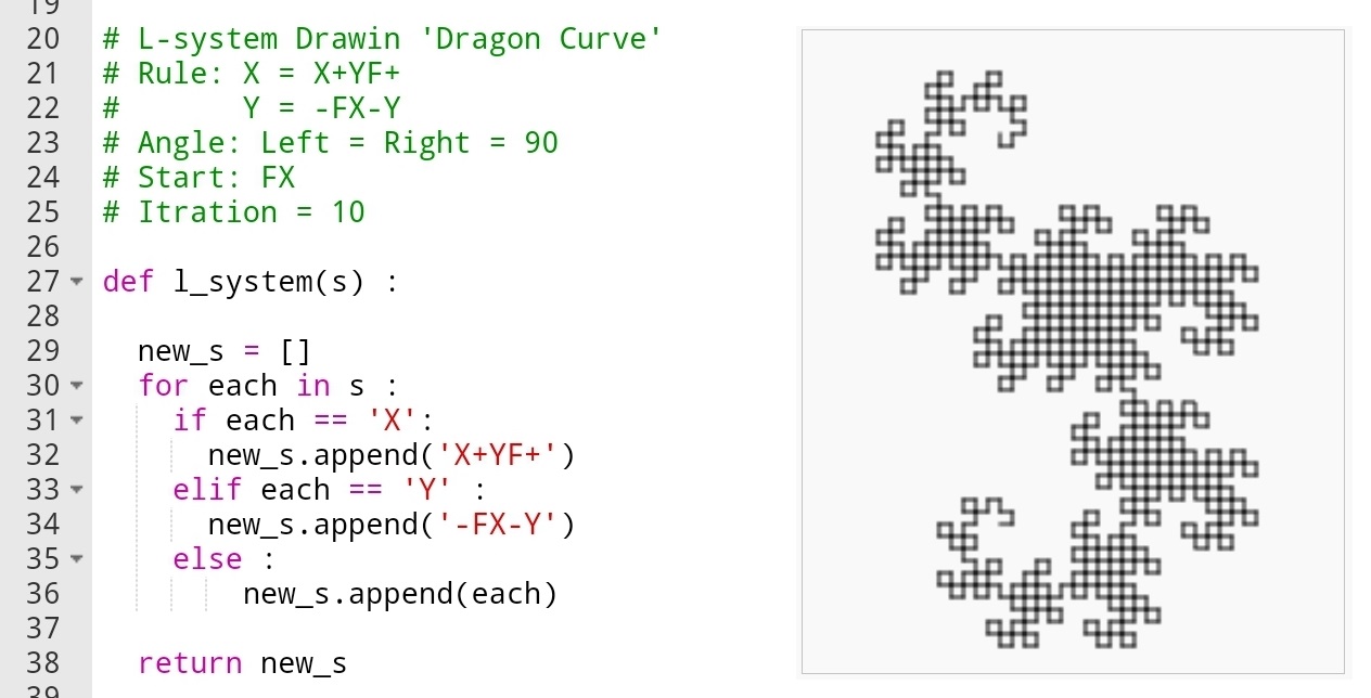 |
L-System: Koch Snowflake 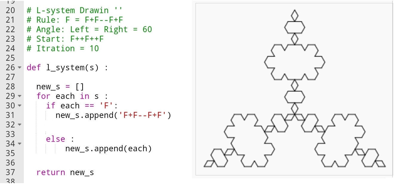 |
L-System: 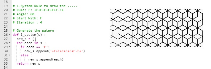 |
L-System:  |
The possibilities to generate the putters and therefore drawing the output is endless, any slightly changes in the iterations or rotation (+ -) angles will take all output to a new levels. In the coming post, I will use the L-system to generate fractal tree and see what we can get from there.
To Download my Python code (.py) files Click-Here
Taking pictures is not my main daily practices, but when i start playing with my camera, i really enjoy my self.
Thanks for visiting my Space..


