Archive
Library System with Excel -P4
Learning :Excel formulas and VBA Cods
Subject: To Develop a Library System with Excel
In last post we wrote all the codes needed to Manage the Authors.
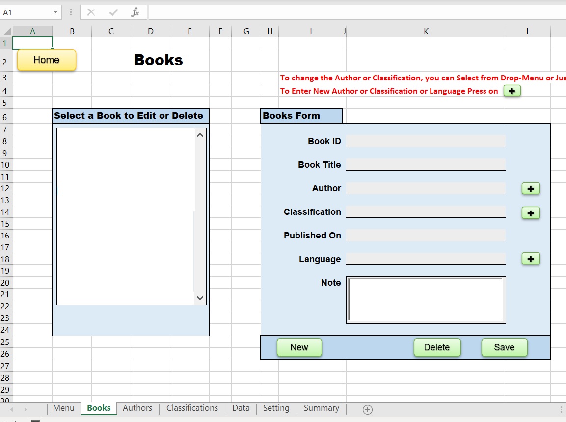
In this part we will do all the coding needed to enter New Books and Edit or Delete anyone we select, in Classifications and Authors we were dealing with one attribute, but here with Books Manage form we have several pieces of information to collect from the user such as [Book Title, Book Author, Book Classification, Publish date, Notes, Book Language ]. So first let’s design the form..
1. Open the Books sheet
2. Change the color of the range(B6:E24)
3. In Cell B6 write “Select a Book to Edit or Delete”, Color and format it as you want.
4. In Cell H6 write “Books Form”, Color and format it as you want.
5. Color and format the Range (B6:L26) as you want.
6. Create three rectangular shapes as New, Delete, and Save buttons.
7. Create another three small rectangular shapes write “+” inside them.
5. We need to create a ListBox name it “books_ListBox 4”.
6. Arrange everything as in the image.
 |
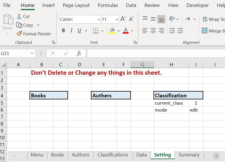
Now move to the “setting” sheet and write the following: B4:Books, B5:current_book, C5:1, B6:mode, C6: edit.
Then in the “Data” Sheet starting from A1 write the following:
A1:Books Data, B1:BookTitle, C1:book_author, D1:class, E1:Published, F1:Note, G1:lang
A2:ID, B2:Title, C2:Author, D2:Class, E2:Published, F2:Note, G2:language
CODING:
To copy the list of the Books we have into the books_ListBox 4 we create:
1.1 From the Menu go to Formulas and click on Name Manager.
1.2 From the pop-up screen click on New, then write books_list in Name, and =OFFSET(Data!$B$3,,,COUNTA(Data!$B:$B)) in Refers to.
2.1. Select books_ListBox 4 on the Books sheet.
2.2. Right-click the mouse, and select FormatControl.
2.3. Goto Control Tab, and in Input range write: books_list, and in Cell link write Setting!$C$5 then press OK.
Now the listBox will contain the Books we have in the Books table in Data Sheet. (If we have any Data there)
3. Data Validation: We need to create Data Validation-list in the cells K12: for Authors list, K14: for Classifications list and K18: for Language list.
1. Select K12, from Data-menu click on Data-validation, select List then in the source type this: =OFFSET(Data!$K$3,,,COUNTA(Data!$K:$K))
2. Select K14, from Data-menu click on Data-validation, select List then in the source type this: =OFFSET(Data!$P$3,,,COUNTA(Data!$P:$P))
3. Select K18, from Data-menu click on Data-validation, select List then in the source type this: =OFFSET(Data!$M$3,,,COUNTA(Data!$M:$M))
book_new_Click() In this function we will Clear all cells [k8, k10,k12,k14,k16,k18, K20] also the note_TextBox1 and will change the cell C6 in Setting Sheet to “new”. Here is the code..
‘ Clear all cells.
Sheets(“Books”).Range(“K8”).Value = “” ‘ID/number
Sheets(“Books”).Range(“K10”).Value = “” ‘Title
Sheets(“Books”).Range(“K12”).Value = “” ‘Author name
Sheets(“Books”).Range(“K14”).Value = “” ‘classification
Sheets(“Books”).Range(“K16”).Value = “” ‘published date
Sheets(“Books”).Range(“K18”).Value = “” ‘language
Sheets(“Books”).Range(“K20”).Value = “” ‘note
Sheets(“Books”).note_TextBox1 = “”
‘ change book mode to “new”
Sheets(“setting”).Range(“c6”).Value = “new”
Sheets(“Books”).Range(“K8”).Select
End Sub
now in the Books sheet select the button “New” we create and assign the “book_new_Click” macro to it.
book_save_Click() The Save function will have tow parts, if the user click on New then we will have:
Sheets(“setting”).Range(“C6”).Value = “new” in this case we will copy all the Book Data from Range(“K8”),Range(“K10”),Range(“K12”),Range(“K14”),Range(“K16”),Range(“K18”) and the value of the note_TextBox1 to the Data sheet under Boos Table, then will empty all the range in the book form, also will pop-up a MsgBox ” One New Book has been Added.”.
if Sheets(“setting”).Range(“C6”).Value = “edit” in this case we will get the current selected book location by selected_book = Sheets(“setting”).Range(“C5”).Value + 2 then re-copy the book data from the form to the Book Table in the Data Sheet and pop-up MsgBox ” One Book Data has been Updated.”.
In Books form we have also three + buttons next to Author, Classification and Language cells, if the user did not find say the Author in the list then he/she can add new one by clicking on the +
Edit Book Data: The user can select any Book from the Book List on the left-hand list then it’s Data will show-up in the form, the user then can change any of the Book-Data and press on Save.
book_delete_Click() The user will select the Book to de deleted then click on “Delete” button, a massage will pop-up to make sure that Book will be DELETED, if the user confirm the cation (press OK) we will run this line of code:
‘To get the book row number.
selected_book = Sheets(“setting”).Range(“C5”).Value + 2
‘To delete the book row
Sheets(“data”).Range(“A” & selected_book & “:G” & selected_book).Delete Shift:=xlUp
Pressing the (+) button: We have three (+) buttons in this form to add New Authors, Classifications, and Languages if not exist in the list; for example, if the user couldn’t find the Author of the Book (he/she want to enter to the system) pressing the (+) will pop-up a dialog box to Enter New Author and the same for classification and Language. Here is the code..
Sheets(“Books”).Range(“K12”).Value = “”
new_author_name = InputBox(“Enter a New Author Name and Click OK:”, “:: New Author :: “)
‘if we add new author then save it.
If new_author_name > “” Then
‘ Get next empty row
next_row = Sheets(“Data”).Range(“K” & Rows.Count).End(xlUp).Offset(1).Row
Sheets(“Data”).Range(“K” & next_row) = new_author_name
Sheets(“Books”).Range(“K12”).Value = new_author_name ‘Author name
Sheets(“setting”).Range(“F6”).Value = “still”
‘ To Sort the Authors list
next_row = Sheets(“Data”).Range(“K” & Rows.Count).End(xlUp).Offset(1).Row
Sheets(“Data”).Range(“K3:K” & next_row – 1).SortSpecial SortMethod:=xlPinYin
End If
Sheets(“Books”).Range(“K12”).Select
End Sub
End of Part-4
Recap this part:
1. We Create the Books header Tabke.
2. We Create a form to collect the Books from the user.
3. We Create the Books ListBox.
4. We wrote the VBA code to Save, Delete, and Create New Book also to retrieve the Books information into Books ListBox.
5. We let the user to Enter New Author, classification, Language into the system through a dialog box.
:: Library System with Excel ::
| Part 1 | Part 2 | Part 3 | Part 4 | Part 5 |
To Download EXCEL (.xlsm) files Click-Here
 Follow me on Twitter..
By: Ali Radwani
Library System with Excel -P3
Learning :Excel formulas and VBA Cods
Subject: To Develop a Library System with Excel
In last post we wrote all the codes needed to Manage the Classifications.
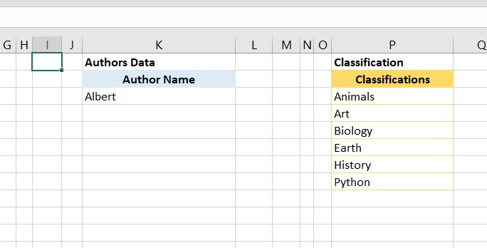
In this part we will do all the coding needed to enter the Authors and Edit or Delete anyone we select, so first we will go to the “setting” sheet and will write the following: E5:current_author, F5:1, E6:mode, F6: edit as in the image.
 |
Now in the “Data” sheets, we create a table with “Author Name” header on range K2, then enter any Autor name such as “Albert” as in the image.
 |
Now, we move to “Authors” Sheet and do the following:
1. In Cell B6 write “Select an Author to Edit or Delete”, Color and format it as you want.
2. In Cell H6 write “Authors Form”, Color and format it as you want.
3. Color and format the Range (B6:E19) and the Range (H6:K13) as you want.
4. Create three rectangular shapes as New, Delete, and Save buttons.
5. We need to create a ListBox name it “authors_ListBox1”.
6. Arrange everything as in the image.
 |
CODING:
To copy the list of the Authors we have into the ListBox:
1.1 From the Menu goto Formulas and click on Name Manager
| |
1.2 From the pop-up screen click on New, then write author_list in Name, and =OFFSET(Data!$K$3,,,COUNTA(Data!$K:$K)) in Refers to [as in image]
 |
2.1. Select the ListBox in the Authors sheet.
2.2. Right-click the mouse, and select FormatControl.
2.3. Goto Control Tab, and in Input range write: author_list, and in Cell link write Setting!$F$5 then press OK.
Now the listBox will contain the Authors we have in the Author list in Data Sheep. … [SEE THE IMAGE]
 |
ListBox Code:
Now we will write a three lines of code to take action when we select any things in this box, so select the ListBox, click right-mouse-button, select “Assinge Macro, then the VBA application will start and write the foloing code:
selected_author = Sheets(“Setting”).Range(“F5”).Value + 2
Sheets(“authors”).Range(“j9”).Value = Sheets(“data”).Range(“K” & selected_author)
Sheets(“Setting”).Range(“F6”).Value = “edit”
End Sub
Buttons Codes:
1. While in Authors sheet, select the rectangular shape named “New”, click right-mouse-button, select “Assinge Macro, then the VBA application will start and we will write this code:
Sheets(“authors”).Range(“J9”).ClearContents
Sheets(“Setting”).Range(“F6”).Value = “new”
Sheets(“Authors”).Range(“J9”).Select
End Sub
2. While the VBA application is on, we will write all the codes we need for Edit and Delete buttons and then will assign the macros:
author_delete_Click
If Not Sheets(“setting”).Range(“F5”).Value Then
MsgBox “Nothing selected to be Deleted..”
Exit Sub
End If
answer = MsgBox(“Are you sure you want to DELETE this Author?.”, vbQuestion + vbYesNo)
If answer = vbYes Then
current_select = Sheets(“setting”).Range(“F5”).Value + 2
Sheets(“Data”).Range(“K” & current_select).ClearContents
next_row = Sheets(“Data”).Range(“K” & Rows.Count).End(xlUp).Offset(1).Row
Sheets(“Data”).Range(“K3:K” & next_row – 1).SortSpecial SortMethod:=xlPinYin
authors_ListBox1_Change
MsgBox “One Author has been Deleted..”
Else
MsgBox “OK, Nothing will be changed.”
End If
End Sub
author_save_Click
If Sheets(“authors”).Range(“J9”).Value = Empty Then
MsgBox “There is no Author Name to Save.”
Exit Sub
End If
If Sheets(“Setting”).Range(“F6”).Value = “new” Then
‘ Get next empty row
next_row = Sheets(“Data”).Range(“K” & Rows.Count).End(xlUp).Offset(1).Row
‘ copy the new classification to the data-table
Sheets(“authors”).Range(“j9”) = StrConv(Sheets(“authors”).Range(“J9”), vbProperCase)
Sheets(“Data”).Range(“K” & next_row).Value = Sheets(“Authors”).Range(“J9”)
‘ Empty the form
Sheets(“Authors”).Range(“J9″).ClearContents
MsgBox ” One New Author Name Saved.”
‘ To Sort the classifications
next_row = Sheets(“Data”).Range(“K” & Rows.Count).End(xlUp).Offset(1).Row
Sheets(“Data”).Range(“K3:K” & next_row – 1).SortSpecial SortMethod:=xlPinYin
authors_ListBox1_Change
Exit Sub
End If
If Sheets(“setting”).Range(“F6”).Value = “edit” Then
selected_author = Sheets(“Setting”).Range(“F5”).Value + 2
Sheets(“authors”).Range(“J9”) = StrConv(Sheets(“authors”).Range(“J9”), vbProperCase)
Sheets(“data”).Range(“K” & selected_author) = Sheets(“authors”).Range(“J9″).Value
MsgBox ” One Author Name Changed.”
‘ Sort the Authors Name
next_row = Sheets(“Data”).Range(“K” & Rows.Count).End(xlUp).Offset(1).Row
Sheets(“Data”).Range(“K3:K” & next_row).SortSpecial SortMethod:=xlPinYin
authors_ListBox1_Change
Exit Sub
End If
End Sub
In the Save code we re-sort the data in the ListBox. Here is a part of the code we use to do so:
‘ Sort the Authors Name
next_row = Sheets(“Data”).Range(“K” & Rows.Count).End(xlUp).Offset(1).Row
Sheets(“Data”).Range(“K3:K” & next_row).SortSpecial SortMethod:=xlPinYin
authors_ListBox1_Change
New we can assign the macros we just creates to the buttons we have (Delete and Save).
End of Part-3
Recap this part:
1. We Create an Author list.
2. We Create a form to collect the Author from the user.
3. We Create the Author ListBox.
4. We wrote the VBA code to Save, Delete, and Create New Author also to retrieve the Author into Author ListBox.
:: Library System with Excel ::
| Part 1 | Part 2 | Part 3 | Part 4 | Part 5 |
To Download EXCEL (.xlsm) files Click-Here
By: Ali Radwani
Library System with Excel -P2
Learning :Excel formulas and VBA Cods
Subject: To Develop a Library System with Excel
In last post we create the sheets and work on the Menus.
In this part we will do all the coding needed to enter the classifications and Edit or Delete anyone we select, so first we will go to the “setting” sheet and will write the following: B4:Books, E4:Authors, H4:Classification as in the image.
 |
Now in the “Data” sheets, we create a table with “classifications” header on range P2, then enter any classification such as “art” as in image.
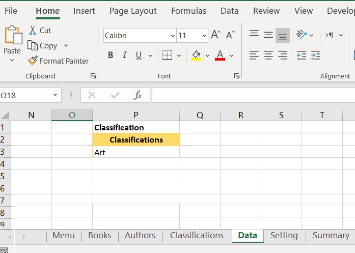 |
Now, we move to “Classification” Sheet and do the following:
1. In Cell B6 write “Select a Classification to Edit or Delete”, Color and format it as you want.
2. In Cell H6 write “Classifications Form”, Color and format it as you want.
3. Color and format the Range (B7:F20) and the Range (H7:M12) as you want.
4. Create three rectangular shape as New, Delete, and Save buttons,
5. We need to create a ListBox name it “class_ListBox1”.
6. Arrange everything as in the image.
 |
CODING:
1. To copy the list of the classification we have into the ListBox:
1.1. Select the ListBox.
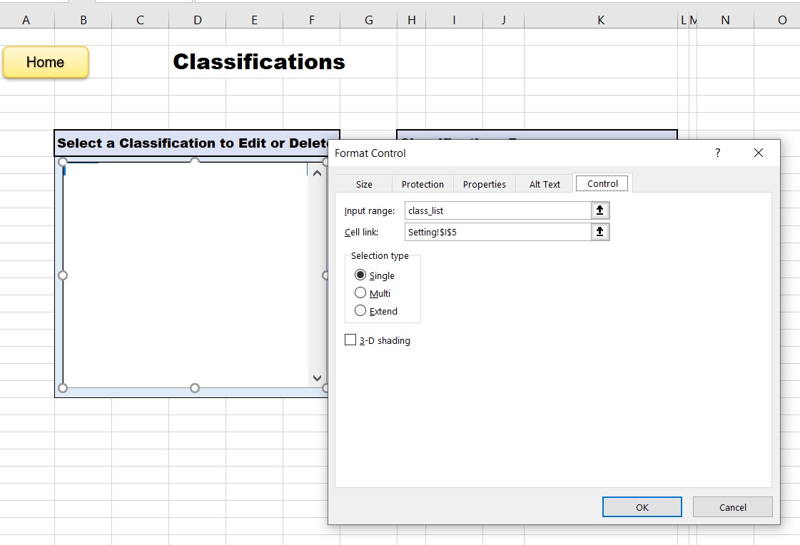
1.2. Right-click the mouse, and select FormatControl.
1.3. Goto Control Tab, and in Input range write: class_list, and in Cell link write setting!$I$5 then press OK.
Now the listBox will contain the Classifications we have in the classification list in Data Sheep. … [SEE THE IMAGE]
 |
ListBox Code: Now we will write a three lines of code to take action when we select any things in this box, so select the ListBox, click right-mouse-button, select “Assinge Macro, then the VBA application will start and write the foloing code:
selected_class = Sheets(“Setting”).Range(“I5”).Value + 2
Sheets(“classifications”).Range(“K8”).Value = Sheets(“data”).Range(“P” & selected_class)
Sheets(“Setting”).Range(“I6”).Value = “edit”
End Sub
Buttons Codes:
1. Select the rectangular shape named “New”, click right-mouse-button, select “Assinge Macro, then the VBA application will start and we
will write this code:
Sheets(“classifications”).Range(“k8”).ClearContents
Sheets(“Setting”).Range(“I6”).Value = “new”
End Sub
2. While the VBA application is on, we will write all the codes we need for Edit and Delete buttons and then will assign the macros:
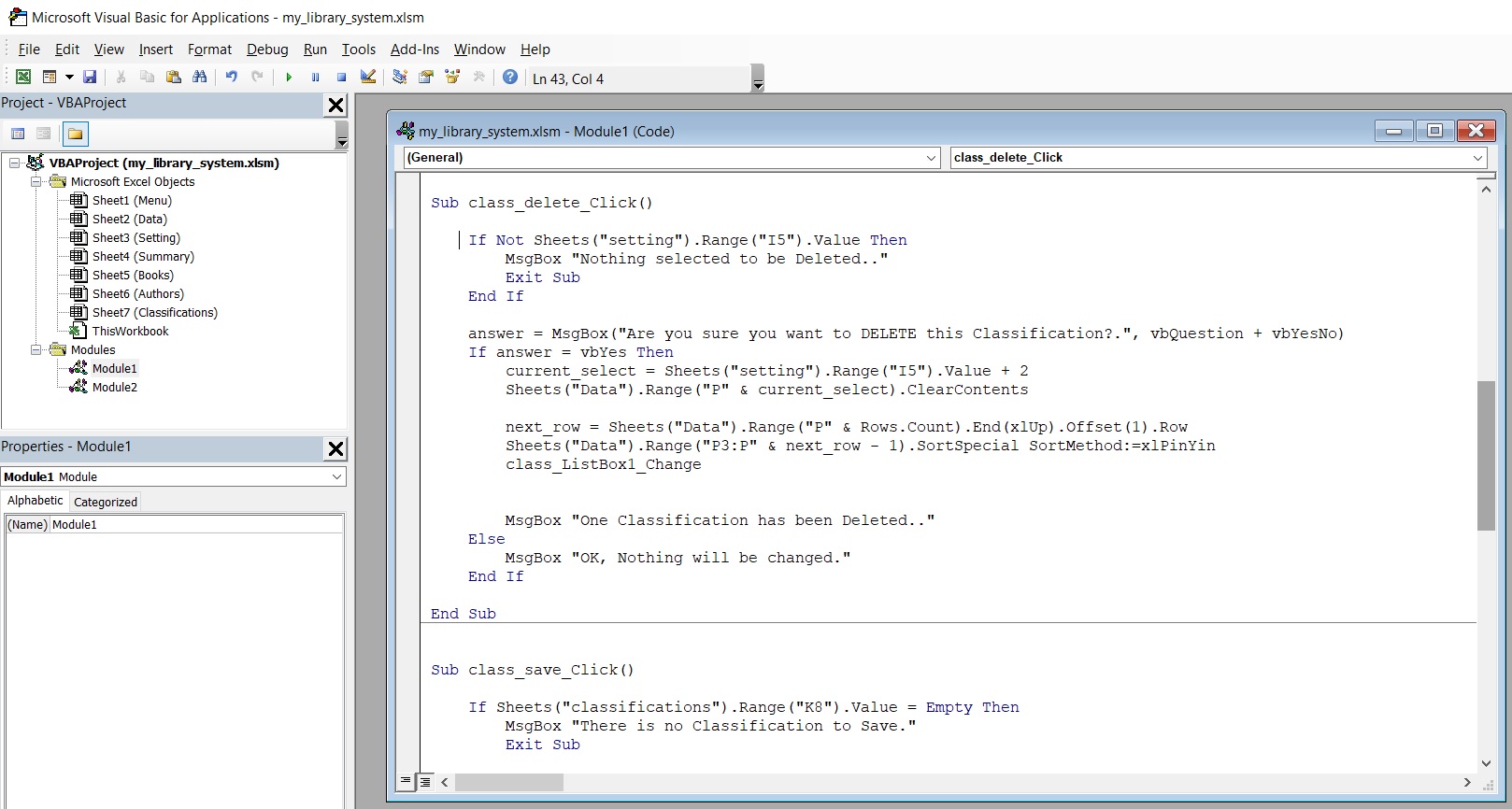
class_delete_Click
If Not Sheets(“setting”).Range(“I5”).Value Then
End Sub
End If
answer = MsgBox(“Are you sure you want to DELETE this Classification?.”, vbQuestion + vbYesNo)
If answer = vbYes Then
current_select = Sheets(“setting”).Range(“I5”).Value + 2
Sheets(“Data”).Range(“P” & current_select).ClearContents
next_row = Sheets(“Data”).Range(“P” & Rows.Count).End(xlUp).Offset(1).Row
Sheets(“Data”).Range(“P3:P” & next_row – 1).SortSpecial SortMethod:=xlPinYin
class_ListBox1_Change
MsgBox “One Classification has been Deleted..”
Else
MsgBox “OK, Nothing will be changed.”
End If
End Sub
class_save_Click
If Sheets(“classifications”).Range(“K8”).Value = Empty Then
MsgBox “There is no Classification to Save.”
Exit Sub
End If
If Sheets(“Setting”).Range(“I6”).Value = “new” Then
‘ Get next empty row
next_row = Sheets(“Data”).Range(“P” & Rows.Count).End(xlUp).Offset(1).Row
‘ copy the new classification to the data-table
Sheets(“Classifications”).Range(“K8”) = StrConv(Sheets(“Classifications”).Range(“K8”), vbProperCase)
Sheets(“Data”).Range(“P” & next_row).Value = Sheets(“Classifications”).Range(“K8”)
‘ Empty the form
Sheets(“classifications”).Range(“k8″).ClearContents
MsgBox ” One New Classification Saved.”
‘ To Sort the classifications
next_row = Sheets(“Data”).Range(“P” & Rows.Count).End(xlUp).Offset(1).Row
Sheets(“Data”).Range(“P3:P” & next_row – 1).SortSpecial SortMethod:=xlPinYin
class_ListBox1_Change
Exit Sub
End If
If Sheets(“setting”).Range(“I6”).Value = “edit” Then
selected_class = Sheets(“Setting”).Range(“I5”).Value + 2
Sheets(“Classifications”).Range(“K8”) = StrConv(Sheets(“Classifications”).Range(“K8”), vbProperCase)
Sheets(“data”).Range(“P” & selected_class) = Sheets(“classifications”).Range(“K8″).Value
MsgBox ” One Classification Changed.”
‘ Sort the classifications
next_row = Sheets(“Data”).Range(“P” & Rows.Count).End(xlUp).Offset(1).Row
Sheets(“Data”).Range(“P3:P” & next_row).SortSpecial SortMethod:=xlPinYin
class_ListBox1_Change
Exit Sub
End If
End Sub
In the Save code we check if the K8 Cell is empty before we save it, and then we also re-sort the data in the ListBox. Here is a part of the code ..
 |
Recap this part:
1. We Create a classification list.
2. We Create a form to collect the classifications from the user.
3. We Create the classification ListBox.
4. We wrote the VBA code to Save, Delete, and Create New classification also to retrieve the classifications into classification ListBox.
:: Library System with Excel ::
| Part 1 | Part 2 | Part 3 | Part 4 |
To Download EXCEL (.xlsm) files Click-Here
By: Ali Radwani
Library System with Excel -P1
Learning :Excel formulas and VBA Cods
Subject: To Develop a Library System with Excel
Someone asked if we can do the Library Management system using Excel, so in the coming several posts we will try to develop an Excel File to store our Books. So I will stop the CRM Project and will work on Library System, we will use MS-EXCEL and VBA code to create a simple spreadsheet looking after our Books.
To start, do the following:
1. We will create an empty Excel file and call it “my Library System” and save it as “Excel Macro-Enabled Workbook.xlsm”
2. Create 7 Tabs(Sheets), name them as:
Menu, Books, Authors, Classifications, Data, Setting, Summary
In this post (Part-1), we will work on the Menu sheet, I will not concern about the themes and colors or fonts all this is back to each user to do formating as needed. So let’s begin with creating four buttons using the insert – shapes Rectangle: Rounded Corners.
 |
We need to create four Rectangle: Rounded Corners, align them as you want and use any theme color, then give each a Captions as in the coming image..
 |
Now, select the Books Button and with Right-Mouse-button select “Assign Macro” and from the new Assign Macro pop-up screen click on New.
 |
This will launch the VBA Application with an open window to write our code, here is the code that if the user clicks on ‘SAY’: Books-Button the Books Sheet will be selected. In coming image, you will find the codes for all buttons we have in the Menu.
 |
Also, we create a code to take us back to the Menu sheets and we call the button MENU, we will add this Button to all sheets we have.
-
Recap this part:
- 1. We Create an Excel file.
- 2. We Create 7 Sheets and named them.
- 3. We Create Buttons for the Menu Sheet.
- 4. We Create the Home Button.
- 5. We wrote the VBA code so we /the user can navigate thrugh the system.
:: Library System with Excel ::
| Part 1 | Part 2 | Part 3 | Part 4 |
To Download EXCEL (.xlsm) files Click-Here
By: Ali Radwani
Excel Simple CRM System P1
Learning : Excel Simple CRM System
Subject: Create Excel Form, Dynamic Name Range and VBA Code to build a simple CRM system.
In this short project we will learn how to create a simple CRM system and and will build forms to collect needed data and store it in tables.
Case Study:
We want to create a simple CRM system to collect data about our employees such as [Name, Department, Salary], we will keep the system (Forms and codes as simple as we can). In this part, we will work on fomrs and code to collect the Employee data.
First, we will open an Excel file, and will create Three Tabs (Sheets), and will name them [Form, Data, Table]. As in figure 1
As in figure 1  |
Now try to create the formes for Employee and another for Departments (Download the Excel file here).
Then in the Data Sheet starting from A1 create a table as A1: Name, B1: Department, C1: Salary, and in the F1 we will create a table named Department List. As in figure 2
figure 2  |
and enter one row of data as in figure 2. Then we also need to create a Dynamic Name Range, for both employee name and Department List, to do so we:
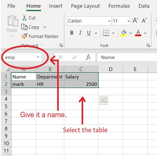
1. Go to Data Sheet.
2. Select the Employee table that we create.
3. in the “NameBox” just give the table a name as “emp”.
Do the same to the Department List table dep_list, we will use these names later.
 |
Coding: Now we will write the VBA code to make a list of Departments we have. To do so we will select the button of SAVE under the Department Form, Click the Right mouse button, and select Assign Macro, then select New and OK, after that the VBA application will start. We will write this code:
Sub save_new_dep()
‘ Get the next empty row
next_row = Sheets(“Data”).Range(“F” & Rows.Count).End(xlUp).Offset(1).Row
Sheets(“data”).Range(“F” & next_row).Value = Sheets(“form”).Range(“J7”)
Sheets(“form”).Range(“J7”).ClearContents
End Sub
figuer 4 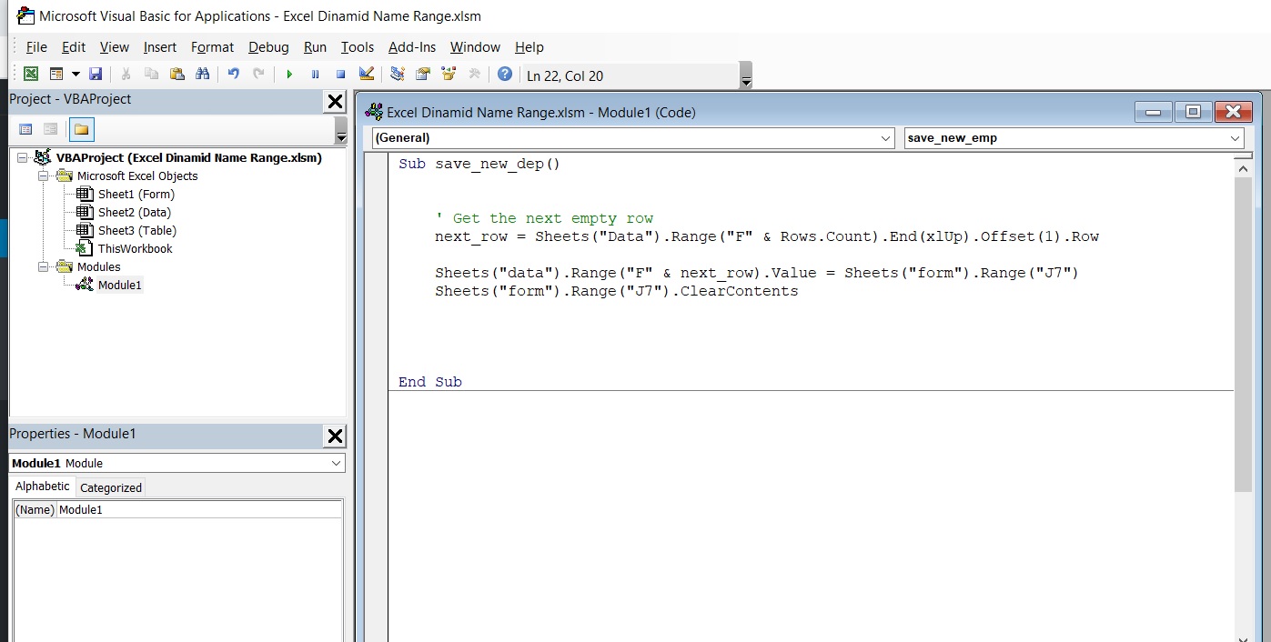 |
In this line
next_row = Sheets(“Data”).Range(“F” & Rows.Count).End(xlUp).Offset(1).Row we will get the next empty row in the department list.
in this line Sheets(“data”).Range(“F” & next_row).Value = Sheets(“form”).Range(“J7”) we will copy the date we just enter as a New Department to the Data Sheet Depatrtment List. Then with Sheets(“form”).Range(“J7”).ClearContents we will clear the content.
So now we can enter some department names: IT, Fin, Economy
We will do the same thing for the Employee Form, so with an open VBA application write the following code. as in figure 5
Sub save_new_emp()
‘ Get the next empty row
next_row = Sheets(“Data”).Range(“A” & Rows.Count).End(xlUp).Offset(1).Row
‘ Copy the Data
Sheets(“data”).Range(“A” & next_row).Value = Sheets(“form”).Range(“D7”)
Sheets(“data”).Range(“B” & next_row).Value = Sheets(“form”).Range(“D8”)
Sheets(“data”).Range(“C” & next_row).Value = Sheets(“form”).Range(“D9”)
‘ Clear the Form
Sheets(“form”).Range(“D7”).ClearContents
Sheets(“form”).Range(“D8”).ClearContents
Sheets(“form”).Range(“D9”).ClearContents
End Sub
figure 5 |
The first line of the code is to get the next empty line in the Employee table, then we will use it to copy the data from the form to the data table. In my form, the Name is in D7, the Department in D8, and the Salary in D9. here is the code line for the name: Sheets(“data”).Range(“A” & next_row).Value = Sheets(“form”).Range(“D7”), then we clear the form as we did with the Department form. In the Employee form (Range”D9″) we need to make it as a DropDown list of all Departments we have so we can select from the list, to do that follow the coming steps ..
1. Select Cell D9.
2. From the Menu Select Data then Data Validation, a popup box will apear as in figure 6, do as shown, here we will use the Dynamic Name range we create “dep_list” as a source. figure 6
figure 6  |
At this point we have two Forms, one for the Department List and one for the Employee (Name, Department, Salary), both forms has SAVE buttons, the Data will be saved in the Data Sheet
To Download Excel files Click-Here
By: Ali Radwani
Excel : Form to Save Data P-1
Learning : VBA Codes to Save Data
Subject: Create Form to collect Data
In a very fast and as simple as we can, we will design and write VBA codes to transform three fields of Data from an Excel sheet “Form” to another sheet “Data”.
To keep thing as simple as we can, we will not use any Validations on user inputs in this example.
First, we will re-name a sheet to “Form” and another one to “Data”. In sheet [Form] we will create a simple Form to collect Names, Company Name and Emails of our customers, also we add a button and call it Save. As in Image-1
Image-1 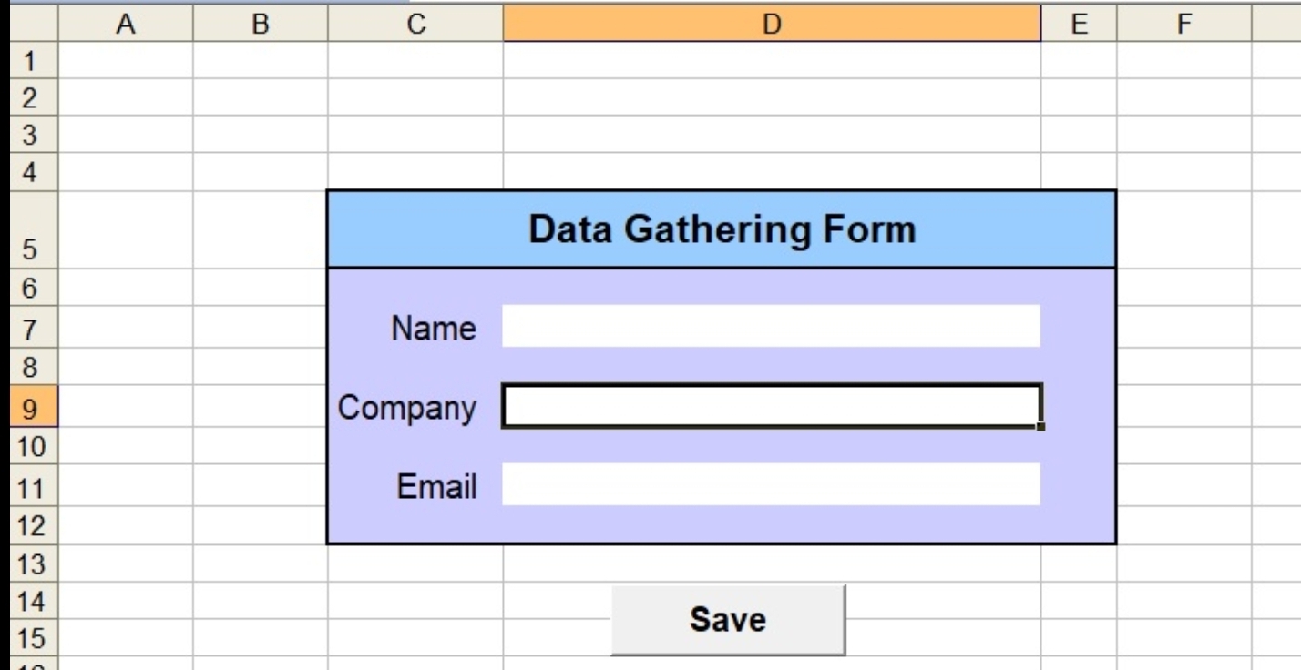 |
For companies Name, We will create a list then we will link it to Cell”D9″ so we can select a “Company Name” from a drop-down list. So to do this First in the Data sheet I will write a list of companies Name as (Comp Name 1,Comp Name 2,Comp Name 3, …. to Comp Name 10). I start my list from Cell “H8” [As in Image-2] you may start from any Cell you want.
Image-2 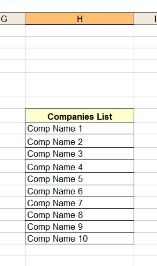 |
Now to link a Dropdown list of our companies Name to Cell “D9″ Do this:
1. Goto Cell”D9”.
2. From the menu we will select “Data” then “Data Validation” and select Data Validation. [Image-3]
Image-3 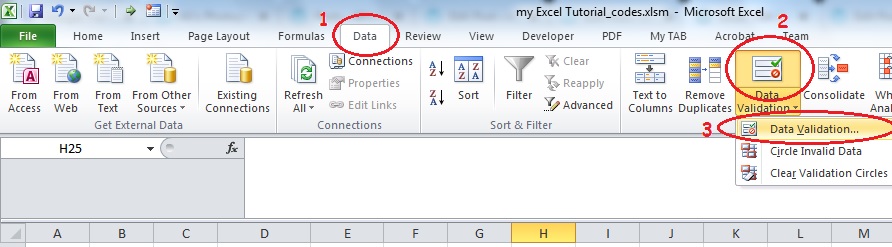 |
3. In the Allow [Select “List”], then in the Source we select the range of Companies we write [Range Cells H8:H17] or just write this: =$H$8:$H$17. Then click OK. See Image-4
Image-4 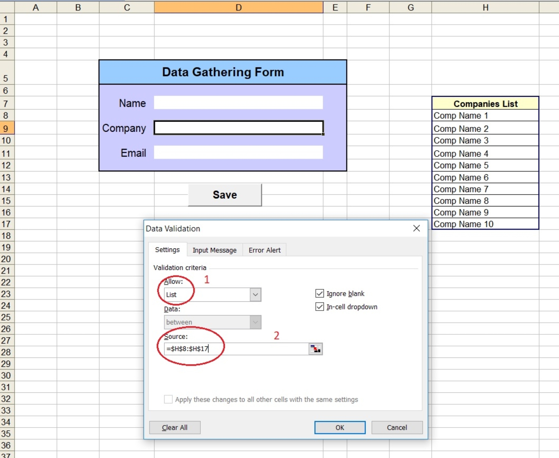 |
Now if we try to click on Cell “D9” we will have a list as in Image-5.
Image-5 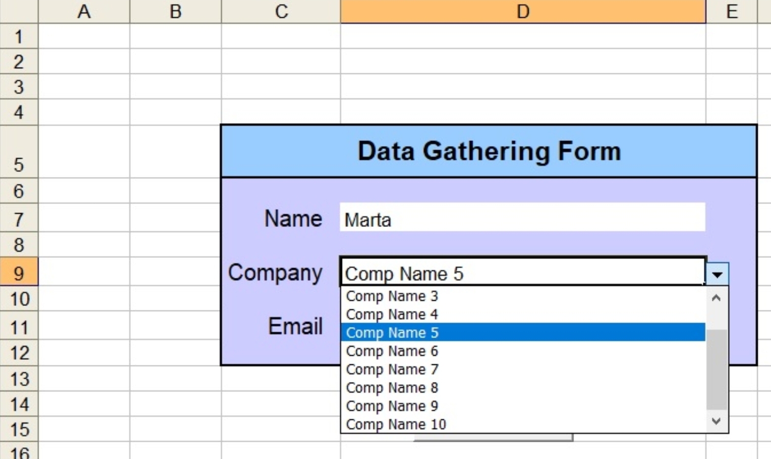 |
In the “Data” Sheet we will just create the Table Header as in Image-6, and will go-back to “Form” Sheet.
| Image-6 |
Now we will write the VBA codes and link it to to a “Save” Button we create. To open the Visual-Basic window we select “Developer” From the Top menu, then Press Visual Basic.
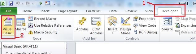 |
Then we write this code and link it to the Save Button. ..
 # VBA Macro code to Save Data to Data sheet

Sub Save_data()
'
' Save_data Macro
' Macro recorded 2020-03-29 by HP
'

'
    ' Set Variables
    Name = Range("D7").Value
    comp_name = Range("D9").Value
    Email = Range("D11").Value


    ' Goto data sheet
    Sheets("Data").Select
    ' This line will get the Next empty Row in the Data sheet.
    emp_row = Range("A" & Rows.Count).End(xlUp).Offset(1).Row
    Range("A" & emp_row).Value = Name
    Range("B" & emp_row).Value = comp_name
    Range("C" & emp_row).Value = Email

    'Go to Form Sheet.
    Sheets("Form").Select

    ' Clear data cells.
    Range("D7").Value = ""
    Range("D9").Value = ""
    Range("D11").Value = ""

    Range("D7").Select

End Sub
Now if we enter some data [as we said: No Validation on the data] and press the Save button, the data will be coped to next empty row in the Data Sheet.
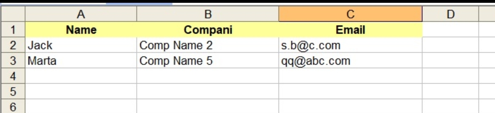 |
Enhancement: In some cases as in our coming project, it’s better to create a sheet and call it “Setting”, then we can have our Lists (such as Company-Name), Colors, Filters all to be in the Setting sheet. [We will see this in the Next Project.]
By: Ali Radwani
Excel, VBA Codes and Formulas-4
Learn To : In Excel – Highlight the Row when clicked.
Assume we have a table, and all we want to do is that if the user click anywhere in the table that ROW will change it’s color.
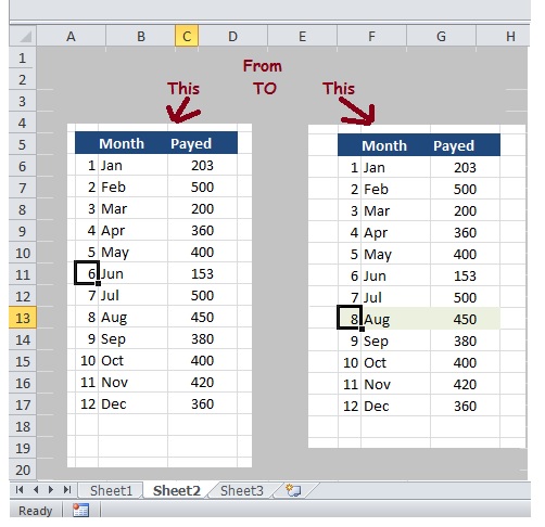 |
Steps
1. From the Top menu, Go to “Developer”, then Press Visual Basic.
| |
2. from the select the sheet name containing the table. ( We have it in Sheet 2 )
3. Then we select “SelectionChange” action from the
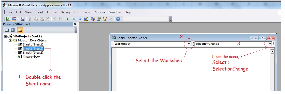 |
4. Write this code:
If Not Intersect(ActiveCell, Range(“C8:E9999”)) Is Nothing Then
Range(“A1”).Value = Target.Row
End If
5. You need to know your Table Range, in my example, the range is (“C8:E9999”). I add the “9999” so i will be sure the even if we add more data to out Table the code will handle it.
6. Now we need to add a rule in the “Manage Roles” in “Conditional Formatting” from the Excel Menu. Here is how to Open it.
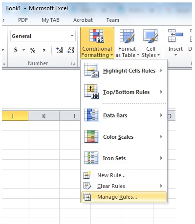 |
7. Select the “” then add new Rule, Follow the Image showing the steps to do that. Once we finish it should work fine.
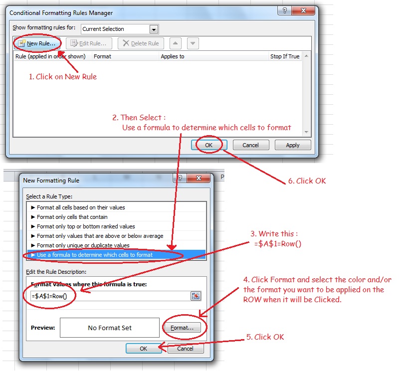 |
Now, when the user click any cell in the Table the Row will change it’s color (Format) as we set it.
🙂 Have Fun ..
By: Ali Radwani
Excel, VBA Codes and Formulas-1
Learn To : In Excel – Drop Down List in a cell.
I start working on a project for a friend, he has some requests to be done on a MS-Excel, so I thought why not to write several posts about MS-Excel capabilities.
MS-Excel is a great application to be used, I will not write to praise the program, but will jump to coding. In Excel we can use dozens of built in ready to use tools and Formulas. Also MS-Excel has a very good, easy to use and learn programming language called VBA (Visual Basic for Application) which with simple code we can perform some tasks and create Menus, buttons and functions that runs in background.
Starting from this post we will use some built-in functions and VBA’s one that I am using in my Excel files.
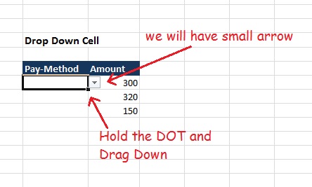
So let’s say we have a table that has a column called “Pay-Method”, the value we save in this column always is one of three: “Cash, Card, Cheque” we don’t want the user to type it every time, but to select it from a list.
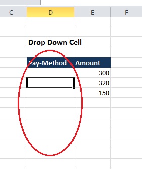 |
To do this we can use an static approach or a Dynamic approach.
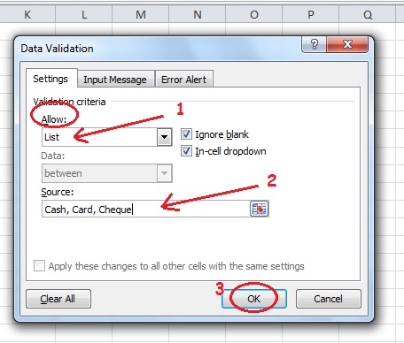
Static Approach: if we have a specific answers that can’t be more like (Yes,No) or as our example above (Cash, Card, Cheque) or similar cases then we can use an static approach. So First Select First cell in the Table, from the menu we will select “Data” then “Data Validation” and select Data Validation.
| |
Now,
- From the Allow box, we select List.
- Then in Source box, we need to type the items we want to appear in each cell as a drop-down list separated by a comma. Cash, Card, Cheque
- We need to check [Ignore Blank and In-cell Dropdown] Then Click OK.
 |
Now we will have a small arrow on the first cell in our Table, to copy the List to other Cells (Beneath) hold the small DOT and Drag it down.
 |
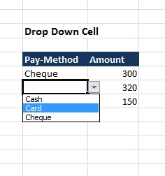
And Now we are DONE, we just create a Dropdown List in all “Pay-Method” Column in the table..
 |
Dynamic Approach: If we have a list of items and this list is growing (We may add more items ti it), such as Fruit list in a grocery, then we will use the Dynamic drop-down list. In this case I prefer to use a new Excel Tab call it “Setting”, so we will create one. On that Tab create a Table call it “Fruit” and list all the fruits you want to be appear in the drop-down cell list (In this example I will list down F1, F2, F3, F4, F5), Select the table and from Menu select “Format as Table” and just chose any format you want. Here is a screen shot.
Here is a screen shot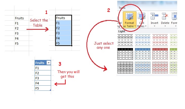 |
Move the Mouse next to table head until you get small Arrow, and give it a name. as in here..
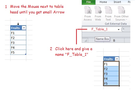 |
Now go-back to our main Table and using the same way we did in the Static Approach (from the menu we will select “Data” then “Data Validation” and select Data Validation.) AND
- From the Allow box, we select List.
- Then in Source box, we need to type the Name we select for our table “F-Table_1” for the fruit table
- We need to check [Ignore Blank and In-cell Dropdown] Then Click OK.
Done … Now if we add new Fruit to the list “F6” it will appear in our Drop-Down cell list.
🙂 Have Fun ..
By: Ali Radwani
My Fitbit Data
Solving My Fitbit data Problem
Subject: VBA code to combine Fitbit excel files into one
I purchase a Fitbit Alta HR in 2017, and since then I wear it and never take it off unless for charging. Fitbit Alta HR is a very nice slim device, but unfortunately there was no way to upload my previous data from my old device to my Fitbit, this was not the only issue with Fitbit data, now; after three years still we can’t download Fitbit data in one file, if you want to do this (each time) you need to send a request to Fitbit team and they will prepare the file for you!! Instead, Fitbit site allow you to download your data as month by month, in my case I will have almost 32 files.
Solving the Problem: After downloading the excel files and look at them, I decide to write a code to help me combine all the current 32 files and any coming once into one data file. First I start thinking to use Python to do this task, but after second thought I will use the Excel file and VBA macro coding to do it.
Here in coming paragraph I will post about the general idea and some codes that i use.
General Idea: I will use same structure of Fitbit file and name it as “fitbit_All_data_ali”, in this file we will create new tab and name it Main. In the Main tab we will create several buttons using excel developer tools and will write the macro VBA code for each task we need to operate.
Tabs in our file: Main: Contain buttons and summary about my data.
Body, Food, Sleep, Activities and Food Log. Food Log tab will store the data such as calories, fibers, fat and so-on., all those tabs will be filled with a copied data from each Fitbit data file.
Here are some VBA codes that I use and what it’s purpose .
| Code: ‘ Get current path. the_path = Application.ActiveWorkbook.Path |
The path on the current excel file. |
| Code: the_All_Data_file = ThisWorkbook.Name |
Get current excel file name |
| Code: Workbooks.Open Filename:=thepath + my_source_Filename |
Open a file |
| Code: Windows(my_source_Filename).Activate Sheets(“Foods”).Select Range(“A2:B31”).Select Selection.Copy |
Goto fitbit file, goto food sheet, select the data copy it. |
| Code: Application.CutCopyMode = False Workbooks(my_source_Filename).Close SaveChanges:=False |
Close an open excel file. |
| Code: Range(“A3”).Select Selection.EntireRow.Insert , CopyOrigin:=xlFormatFromLeftOrAbove |
To insert a black Row |
| Code: sname = ActiveSheet.Name |
Get current sheet name |
| Code: Function go_next_sheet() As String ‘ This code will go to next sheet if there is one, if not will return ‘last’ On Error Resume Next If sht.Next.Visible xlSheetVisible Then Set sht = sht.Next sht.Next.Activate End Function |
if there is no more tabs or sheets, function will return “last” |
Final Results: After i run the code, I have an Excel file contain all my Fitbit data in one place. Mission Accomplished
To Download my Python code (.py) files Click-Here
Taking pictures is not my main daily practices, but when i start playing with my camera, i really enjoy my self.
Thanks for visiting my Space..


