Archive
Excel, VBA Codes and Formulas-2
Learn To : In Excel – SUMIF and SUMIFS [ Part-1 SUMIF ]
Case Assumption: Assume we have a table, with 5 columns (as in image-1) columns titles are [Date, Item, Quantity, Price and Total] containing our Expendituer and we have another table call it Summaries, we want some totals to be in this table. In Image-1 we can see the main table [Expendituer] and the Summary table.
Image-1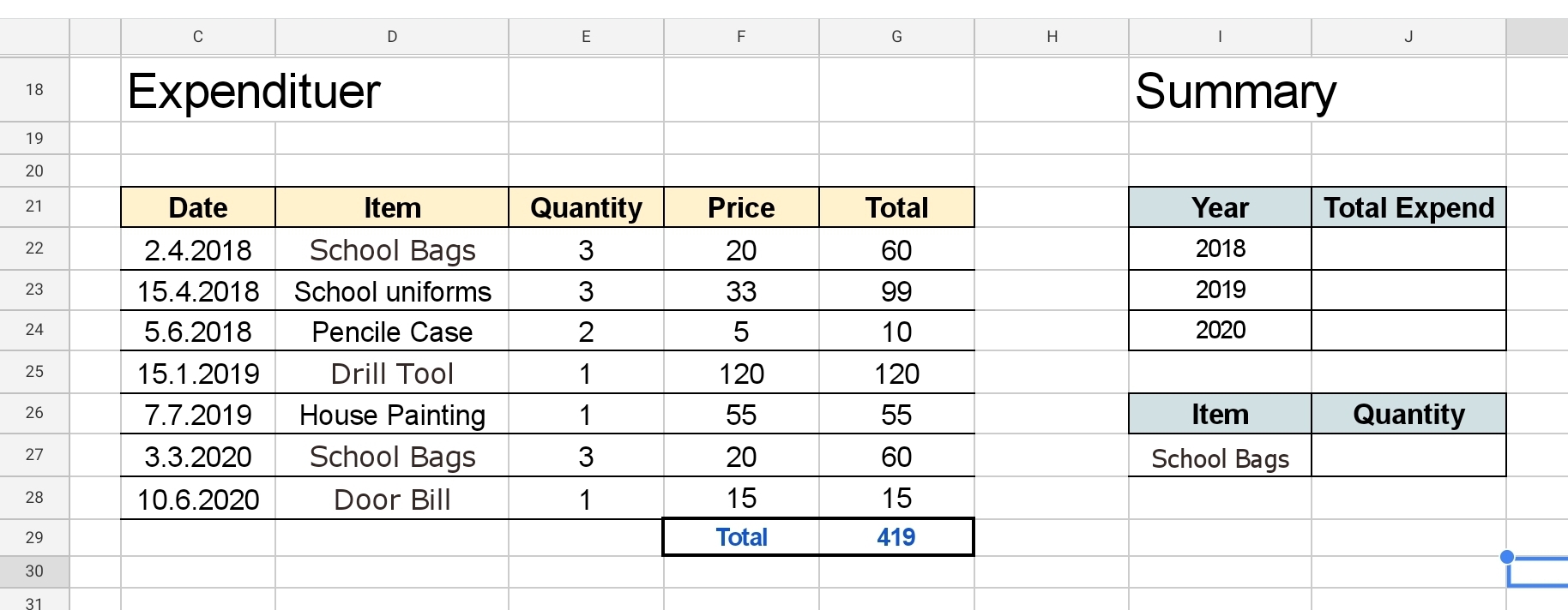 |
In the Above Expendituer Table we have some [Dummy] data, and in our Summary Table we want to calculate the SUM of each year so in the Cell J22 we shall write this formula: =SUMIF()
SUMIF will take 3 parameters First one is the range of applying the condition. Second one is the condition. Third one is the range to calculate to SUM form. So in our case [Image-1]
The range of applying the condition will be C22:C28
The condition is in Cell I22 [23,24,25 … for each row and year.]
The range to calculate to SUM form will be G22:G28
So in Cell J22 we will write =SUMIF(C22:C28,”*”&I22,G22:G28)
then we can copy the formula to other cells [I23 and I24]
So now we have the Sum in each Year. See Image-2
Image-2 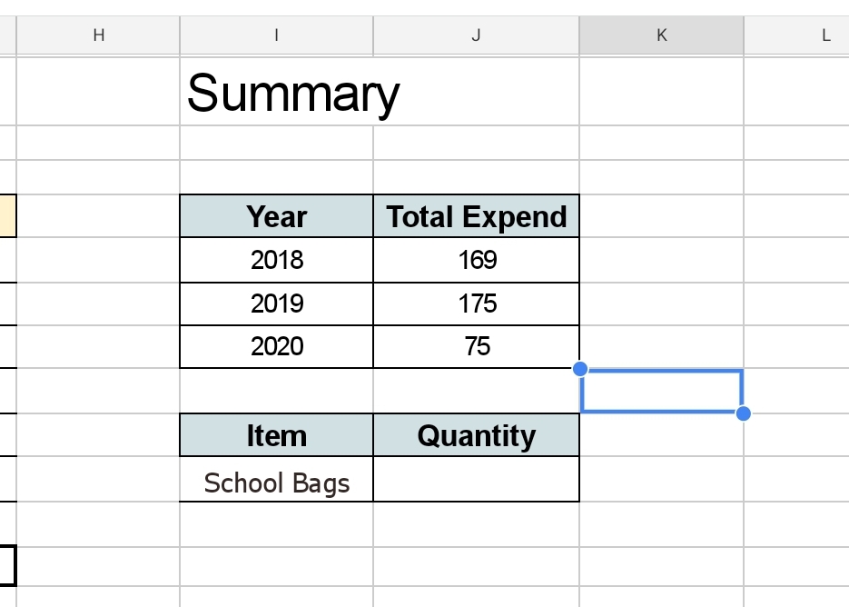 |
Now with same formula SUMIF, we can get the Quantity of each Item we purchase, and we will write the formula in Cell J27 [as in Image-1].
So in Cell J27 we will write =SUMIF(D22:D28,I27,E22:E28) as in Image-3 then we copy the formula to Cells [J28, J29, J30 .. and so]
Image-3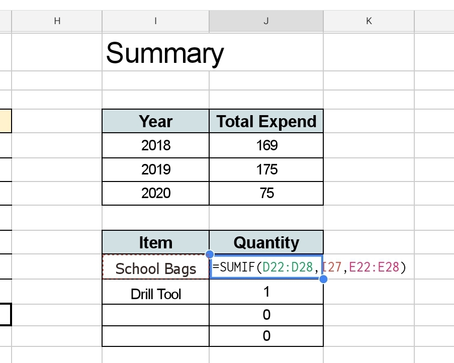 |
Now we have the sum of Quantity.
🙂 Have Fun ..
 Follow me on Twitter..
By: Ali Radwani
Excel, VBA Codes and Formulas-1
Learn To : In Excel – Drop Down List in a cell.
I start working on a project for a friend, he has some requests to be done on a MS-Excel, so I thought why not to write several posts about MS-Excel capabilities.
MS-Excel is a great application to be used, I will not write to praise the program, but will jump to coding. In Excel we can use dozens of built in ready to use tools and Formulas. Also MS-Excel has a very good, easy to use and learn programming language called VBA (Visual Basic for Application) which with simple code we can perform some tasks and create Menus, buttons and functions that runs in background.
Starting from this post we will use some built-in functions and VBA’s one that I am using in my Excel files.
So let’s say we have a table that has a column called “Pay-Method”, the value we save in this column always is one of three: “Cash, Card, Cheque” we don’t want the user to type it every time, but to select it from a list.
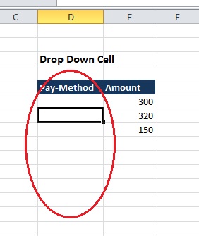 |
To do this we can use an static approach or a Dynamic approach.
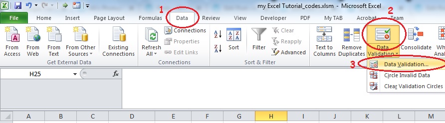
Static Approach: if we have a specific answers that can’t be more like (Yes,No) or as our example above (Cash, Card, Cheque) or similar cases then we can use an static approach. So First Select First cell in the Table, from the menu we will select “Data” then “Data Validation” and select Data Validation.
 |
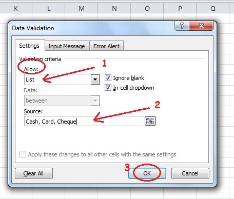
Now,
- From the Allow box, we select List.
- Then in Source box, we need to type the items we want to appear in each cell as a drop-down list separated by a comma. Cash, Card, Cheque
- We need to check [Ignore Blank and In-cell Dropdown] Then Click OK.
 |
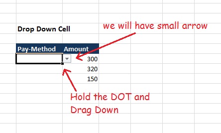
Now we will have a small arrow on the first cell in our Table, to copy the List to other Cells (Beneath) hold the small DOT and Drag it down.
 |
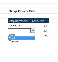
And Now we are DONE, we just create a Dropdown List in all “Pay-Method” Column in the table..
 |
Dynamic Approach: If we have a list of items and this list is growing (We may add more items ti it), such as Fruit list in a grocery, then we will use the Dynamic drop-down list. In this case I prefer to use a new Excel Tab call it “Setting”, so we will create one. On that Tab create a Table call it “Fruit” and list all the fruits you want to be appear in the drop-down cell list (In this example I will list down F1, F2, F3, F4, F5), Select the table and from Menu select “Format as Table” and just chose any format you want. Here is a screen shot.
Here is a screen shot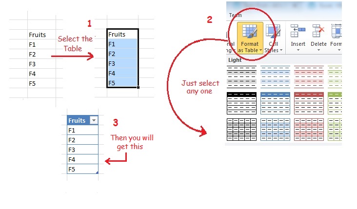 |
Move the Mouse next to table head until you get small Arrow, and give it a name. as in here..
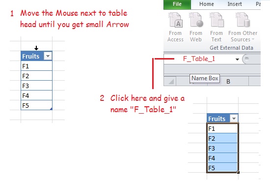 |
Now go-back to our main Table and using the same way we did in the Static Approach (from the menu we will select “Data” then “Data Validation” and select Data Validation.) AND
- From the Allow box, we select List.
- Then in Source box, we need to type the Name we select for our table “F-Table_1” for the fruit table
- We need to check [Ignore Blank and In-cell Dropdown] Then Click OK.
Done … Now if we add new Fruit to the list “F6” it will appear in our Drop-Down cell list.
🙂 Have Fun ..
By: Ali Radwani
Taking pictures is not my main daily practices, but when i start playing with my camera, i really enjoy my self.
Thanks for visiting my Space..


